Tool that estimates models' predictive performance using cross-validation
Cross-validation
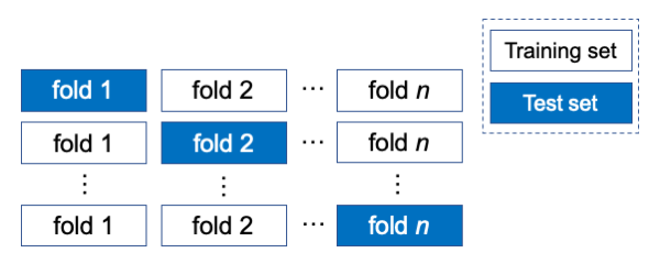
Cross-validation is a resampling procedure used to estimate model's predictive performance on a limited data sample. The procedure takes as inputs a data set and a value of the parameter n. Then, it randomly divides examples from the data set into n folds of approximately equal size. Finally, it repeats n times:
- Hold ith fold as a test set
- Construct a model from the rest of the folds (training set)
- Use the model to annotate examples in the test set
Output
For each ensemble model the cross-validation procedure outputs a table with confidences. Rows in the table are examples, columns are labels (from a hierarchical class) and values are probabilities that the labels are associated with the examples. The probabilities indicate how confident the model is in the established associations. The table aggregates examples from n test sets.
Example
Suppose that we have a simple data set with a tree-shaped hierarchical class of five labels connected in the following manner:
The data set has ten examples. Two-fold cross-validation randomly divides examples in two groups of five: (e2, e3, e7, e9, e10) and (e1, e4, e5, e6, e8). The procedure first constructs a model using the baseline algorithm from the first set of examples and uses the model to make prediction for the second. Then it constructs a model from the second set of examples and makes prediction for the first. The resulting table with confidences is:
| Example ID | Labels | ||||
|---|---|---|---|---|---|
| l1 | l2 | l3 | l4 | l5 | |
| e1 | 0.12 | 0.87 | 0.05 | 0.61 | 0.79 |
| e2 | 0.98 | 0.05 | 0 | 0 | 0.01 |
| e3 | 0.02 | 0.59 | 0.05 | 0.24 | 0.59 |
| e4 | 0 | 0.99 | 0.81 | 0.33 | 0.4 |
| e5 | 0.31 | 0.55 | 0.12 | 0.05 | 0.01 |
| e6 | 0.19 | 0.91 | 0.88 | 0.02 | 0 |
| e7 | 0.84 | 0.12 | 0.01 | 0 | 0 |
| e8 | 0.14 | 0.74 | 0.09 | 0.71 | 0.73 |
| e9 | 0.31 | 0.89 | 0.27 | 0.88 | 0.84 |
| e10 | 0.92 | 0.05 | 0 | 0 | 0.01 |
The table shows which paths from the hierarchy are more or less likely associated with each of the examples. For example, the baseline model is strongly confident in the association between the example e6 and l2 l3 path from the hierarchy (confidence ≥ 0.88).
Note that confidence values for an individual example (within a row) satisfy hierarchy constraint. In other words, confidences for labels do not surpass the confidence of their parent label.
The pipeline has a separate task that divides examples from an input data set (named baseline data set) into n folds. Once the cross-validation folds are created, the pipeline saves the information on which examples are associated with each of the folds. If you want to compare the algorithms on the same cross-validation folds, run this task only once. Then you can run any combination of the algorithms and all of them will be evaluated on the same cross-validation folds.
Measures of model's predictive performance
From the table with confidences the pipeline computes two types of measures of model's predictive performance:
- Threshold-dependent measures set a confidence threshold that differentiates between positive and negative associations of labels with examples. The measures are precision, recall, F-measure and accuracy.
- Threshold-independent measures summarize predictive performance over a range of confidence thresholds. The measures are AUPRC and AUC.
Threshold-dependent measures
Prediction
Suppose that a model predicts a label l for a set of examples. For each example, it will output a confidence. To compute the threshold-dependent measures from the confidences the pipeline follows the steps:
- Set a confidence threshold t
- Associate with l all the examples with confidence for l ≥ t
- Associate with not-l the rest of the examples
Comparison of predicted labels with actual labels
Model's decision to associate l or not-l with an example may or may not be correct. By making such observations over a set of examples, four outcomes can be recorded for the model and the label l:
- True positives (TP) are examples for which the model correctly predicts l
- False positives (FP) are examples for which the model incorrectly predicts l
- True negatives (TN) are examples for which the model correctly predicts not-l
- False negatives (FN) are examples for which the model incorrectly predicts not-l
The outcomes are summarized in a table named confusion matrix:
Actual label Predicted | l | not-l |
|---|---|---|
| l | TP | FP |
| not-l | FN | TN |
Measures
From the confusion matrix, the pipeline compute four measures:
- Accuracy is a share of examples with correct predictions in all of the examples
- Precision is a share of examples with correctly predicted l in the set of examples with predicted l
- Recall is a share of examples with correctly predicted l in the set of examples that are actually associated with l
- F-measure is a harmonic mean of precision and recall
Example
The four threshold-dependent measures are computed for the label l5 and threshold 0.5 by following the steps:
- Prediction: The examples with confidence ≥ 0.5 are associated with l5 and vice versa (the third row in the table):
| Example ID | e1 | e2 | e3 | e4 | e5 | e6 | e7 | e8 | e9 | e10 |
|---|---|---|---|---|---|---|---|---|---|---|
| Confidences for l5 | 0.79 | 0.01 | 0.59 | 0.4 | 0.01 | 0 | 0 | 0.73 | 0.84 | 0.01 |
| Predicted at t = 0.5 | ||||||||||
| Actual label |
- Confusion matrix: Computed by comparing predicted (the third row in the table) and actual labels (the fourth row in the table):
Actual label Predicted | l | not-l |
|---|---|---|
| l | 3 | 1 |
| not-l | 2 | 4 |
- Measures: Computed from the confusion matrix:
- accuracy = 0.7
- precision = 0.75
- recall = 0.6
- F-measure = 0.67
The pipeline outputs a confusion matrix and threshold-dependent measures for each label in a data set. They can be outputted for multiple thresholds. You can define the thresholds in a settings file.
Accuracy is not a good measure of model’s performance in the case of highly unbalanced labels. An example of a highly unbalanced label is when in 100 examples five are labeled with l and 95 as not-l. In such case, a model that would always return not-l as an answer would have 0.95 accuracy. At the same time it would have zero precision, recall and F-measure. Be aware of unbalanced labels in data sets with large hierarchy, where the number of positive examples reduce with the depth of hierarchy.
Threshold-independent measures
Threshold-independent measures indicate model's predictive performance over a range of confidence thresholds. The pipeline implements two such measures: AUPRC and AUC. They are computed for each label and as averages over all labels.
Label-based measures
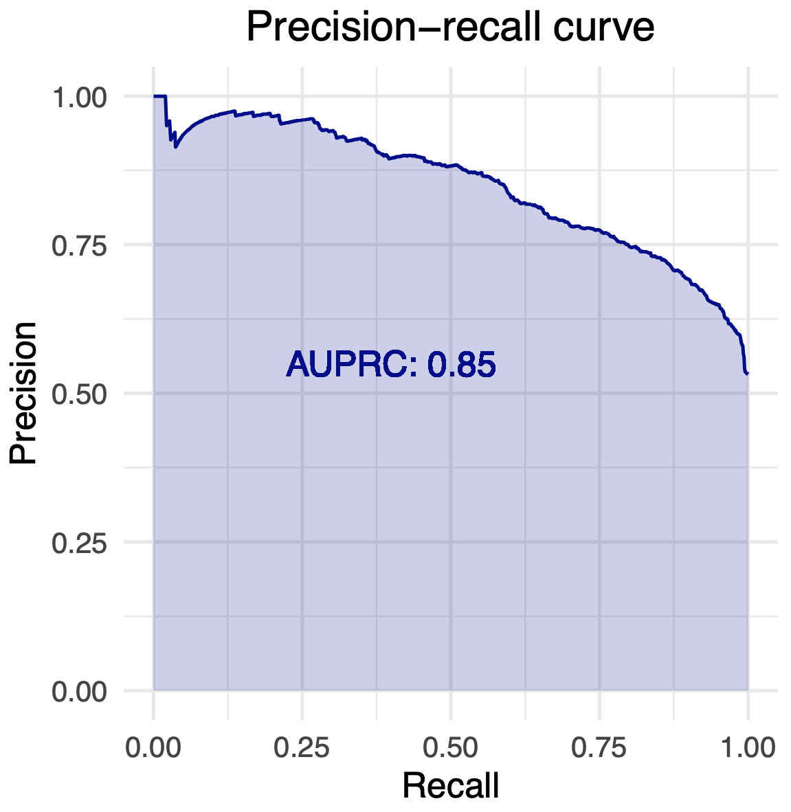
Area under precision-recall curve (AUPRC)
Suppose that a model predicts a label l for a set of examples. AUPRC for l is computed in the following manner:
- Collect thresholds, i.e. a set of distinct confidence values that the model outputted for l
- For each threshold t:
- Compute precision at t
- Compute recall at t
- Draw precision-recall curve where:
- Recall is on x-axis and precision on y-axis
- Points are the values of precision and recall for thresholds
- Curve is drawn using linear interpolation
- Compute AUPRC as an area under the curve.
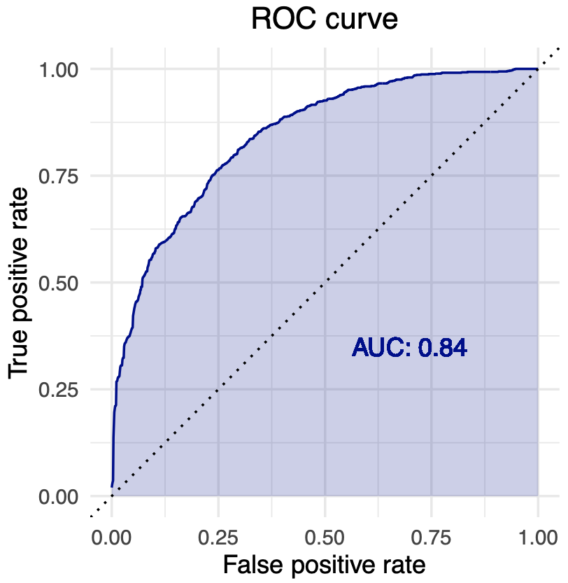
Area under the ROC curve (AUC)
AUC is computed by following the same steps as in the case of AUPRC, with an exception that recall on x-axis is substituted with false positive rate and precision on y-axis with true positive rate.
False positive rate is computed as
\[\text{FPR} = \frac{\text{FP}}{\text{FP + TN}}\]while true positive rate is a synonym for recall.
Measures of overall performance
They summarize model's performance over a set of most specific labels, which are common to all five algorithms. By averaging over the most specific labels, the pipeline ensures fair performance-based comparison between the five algorithms.
The measures are:
- Average AUPRC is an arithmetic mean of label-based AUPRCs computed for labels that qualify as most specific
- Average AUC is an arithmetic mean of label-based AUCs computed for labels that qualify as most specific
- Area under average precision recall curve
Area under average precision recall curve
Suppose that a model predicts a set of most specific labels M for a set of examples. Area under average precision recall curve for M is computed in the following manner:
- For each threshold t ranging from zero to one with the step of 0.01:
- Compute a confusion matrix at t for each label from M
- Compute a micro-average precision as (n is the number of labels in M):
- Compute a micro-average recall as:
- Add the point to a precision-recall graph
- Draw a precision-recall curve using linear interpolation
- Compute area under the curve.
When you run an algorithm in a cross-validation mode, the pipeline will compute the described measures and output them to a file named “Evaluation_report.csv”.